How placement works
The order a layout is built in — usable area, table grid, control rooms, inverters, cables, arresters — and how to read the result in the Layout view.
A layout is built in one pass, in a fixed order. Each stage narrows the ground the next stage is allowed to use, so the order is the design: the boundary becomes a usable area, the usable area is filled with module tables, and every piece of equipment placed after that takes tables back out again.
Knowing the order tells you which input to change when a result is not what you expected. A plant that came out smaller than the site area suggests has usually lost ground at one specific stage — the perimeter road, a transmission line corridor, excluded terrain, or the footprints of the control rooms and arresters — and each of those is a different field on one of the input tabs.
The usable area
Usable area is the ground a module table is allowed to stand on. The plant boundary is shrunk inward by the perimeter road width to give the usable area; obstructions and terrain exclusions are then subtracted.
In full, the usable area is what remains of the boundary after four subtractions:
| Subtracted | Set by |
|---|---|
| The perimeter road band around the inside of the fence | Perimeter road width, on Site parameters |
| Polygon obstructions — water bodies, buildings, substations, and anything you draw by hand | The boundary file, plus Obstructions |
| Transmission line, canal and road corridors, buffered on both sides of the line | Transmission line corridor, per side |
| Ground too steep or too uneven to build on | Topography, when enabled |
Everything placed later is checked against that one area. Tables, control rooms and lightning arresters must sit inside it, and every candidate cable route is validated against it before it is used.
Cables are the single exception to the road band. Cables may run inside the perimeter road band, but never outside the plant fence — the road is a service corridor, not an electrical exclusion.
The road band itself is computed once, as the strip between the boundary and the shrunk boundary, and the same strip is used by the on-screen plot, the report drawing, the Google Earth file and the CAD drawing. The road you see on screen is the road in every export.
The stages in order
1. The boundary file is read
The application reads the plant boundaries out of the file, and with each boundary the obstacles and line features that lie inside it. A polygon that is not contained within another polygon is a plant boundary; a polygon fully contained within a boundary is an obstacle. Which kind of obstacle it is comes from its name, which is why the naming rules in Boundary file requirements decide whether a pond is treated as water or as a plain obstruction.
Several boundaries in one file are laid out as several plants. See Multi-plot sites.
2. Everything is converted to metres
Latitude and longitude are projected into the site's local UTM zone, and all internal geometry from this point on is in metres. Conversion back to latitude and longitude happens only at the edges — when imagery is drawn behind the layout, and when a Google Earth file is written.
This is why every dimension you enter is a length in metres and never an angle or a coordinate: gaps, pitches, footprints, setbacks and radii are all measured on flat ground in the site's own zone.
3. The boundary is shrunk inward by the perimeter road width
The boundary is offset inward by the Perimeter road width — 6.0 m by default — all the way round. What is inside the offset is available for building; the band between the offset and the fence is the perimeter road.
Set the width to 0 and no band is reserved, and tables are then allowed to reach the fence line itself.
4. Obstructions and corridors are subtracted
Every polygon obstacle read from the file is cut out of the area: water bodies, buildings, substations, and any obstruction you draw by hand. Line features are different — a transmission line, canal or road has no width of its own, so each is given a setback on each side of the line. The corridor cut out of the site is therefore twice the setback: at the default Transmission line corridor of 15.0 m per side, a 30 m corridor.
Raise the setback for a higher-voltage line. The application's own tooltip suggests 30 m per side for a 400 kV line.
5. Steep and unsuitable ground is excluded
When Avoid steep ground is on, an elevation model of the site is built — from a contour file you supply, or from public satellite elevation data — and ground that fails your slope limits is cut out of the usable area as well. Ground relief within a single table footprint is limited separately, as the pile-reveal differential you are prepared to build.
Terrain is the one stage that can fail harmlessly. If there is no contour file and no internet connection, the layout proceeds with no terrain exclusion rather than stopping.
6. The table grid is placed
The grid is laid across whatever ground is left. Rows run east to west; panels face the equator — south in the northern hemisphere, north in the southern.
MMS-Tables — modules on a module mounting structure — are laid in rows running east to west, row after row from one edge of the site to the other. Within a row, neighbouring tables are separated by the Gap between MMS-Tables, 1.0 m by default. Row to row, the separation is the Row pitch, which is either the value you enter or the automatic no-shading pitch derived from the site latitude. See Row pitch and tilt.
The table's own dimensions come from the module size, the modules per row and the rows per table — see Table configuration.
7. Only whole tables are kept
A table or tracker unit is placed only where it fits entirely inside the usable area. A position where any part of the footprint crosses the road band, an obstruction, a corridor or excluded terrain is skipped — nothing is clipped, trimmed or half-built.
This rule is what leaves the ragged edge along a diagonal or curved fence: the grid is regular, the boundary is not, and the last position in each row is rejected as soon as one corner falls outside. Two options exist to win that ground back — see Maximizing placement and half tables.
8. Control rooms are placed, and the count re-checked
The plant's capacity is now known, so the number of inverter control rooms (ICRs) follows from it: one room per ICR Block of capacity, 18.0 MWp by default, rounded up. The tables are grouped spatially by position into blocks of roughly one block-size each, and a room is placed at the centre of each group, so every group of tables surrounds its own room.
Each room must fit entirely inside the usable area, and any table overlapping a room's footprint is removed. That drops the plant's capacity — which is why the number of rooms is then re-checked against the new, lower capacity. See Inverter control rooms.
9. Inverters are placed and cables routed
Inverters — or string monitoring boxes (SMBs) in a central-inverter design — are placed from groups of tables, sited in the gap bands between rows rather than in the middle of one. A placed string inverter is drawn as a small marker, 2 m east to west by 1 m north to south. Their counts are reported whether or not cables are routed.
Routing the cables is optional, and it is the slow step on a large or complex
plant. With Calculate cables off — it is on the Cables card of the
Electrical tab, see Cables — the counts still appear and
every cable row of the Summary view reads —. With it on, the DC runs and the
AC runs are routed and measured; the medium-voltage runs to the main control
room follow once that room has been placed and the layout generated again. On a
very large plant the application switches to fast geometric estimation so
generation stays quick. See Cable routing.
10. Lightning arresters are placed, and capacity recomputed
With Place Lightning Arresters on, arresters (LAs) are laid on a coverage grid whose spacing is the protection radius you set, so neighbouring protection circles overlap and no part of the plant is further than one radius from an arrester. On a fixed-tilt plant an arrester has a real footprint and the tables it covers are removed, so capacity falls once more and the plant totals are recomputed. On a tracker plant the arrester is a slim pole placed in the gap between tracker columns, and no units are lost. See Lightning arresters.
With the option off, no arresters are placed at all and tables fill the whole usable area. You can still add them by hand later in Sketch Mode.
Why the order matters
Three of the stages remove tables that stage 6 had already placed: the control rooms, the arresters, and any obstruction you add by hand. Capacity is therefore not final until the last of them has run.
That is the reason for the re-check in stage 8. The number of control rooms is derived from capacity, and capacity is lower after their footprints have been cleared than it was when the count was first worked out. Re-checking against the reduced figure is what stops the plant carrying a room it no longer has the capacity to justify.
Capacity read off the site area will always be higher than the capacity the application reports. The perimeter road, the corridors, the excluded terrain and the equipment footprints are all deducted, and each deduction is a field you control. Compare the two figures before assuming a layout is wrong.
The same logic explains the order of the equipment stages. Control rooms are placed before cables because the cables terminate at them; arresters come last because they are the only equipment whose position is set by coverage geometry rather than by the plant it serves.
Reading the plot
The plot is the Layout view — the first of the five view tabs on the right of the window. How the views, their tools and the chip row fit together is on Views; this section covers what you use to read a layout once it exists.
The tools row
To the right of the view tabs, the Layout view carries its own tools: Save project and Export ▾, then Satellite, Wireframe, Piles: OFF, Layers ▾, Sketch, the Home, Pan and Zoom icons and the expand button.

| Tool | Default | What it does |
|---|---|---|
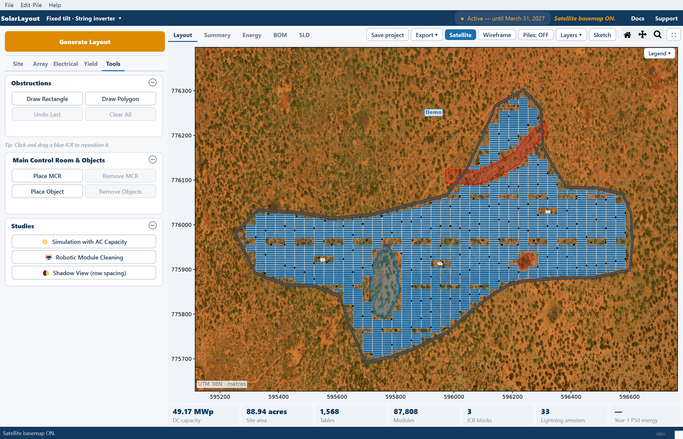
| Satellite | Off, and disabled until a layout exists | Draws an aerial photograph behind the layout, aligned to the file's latitude and longitude. Needs an internet connection |
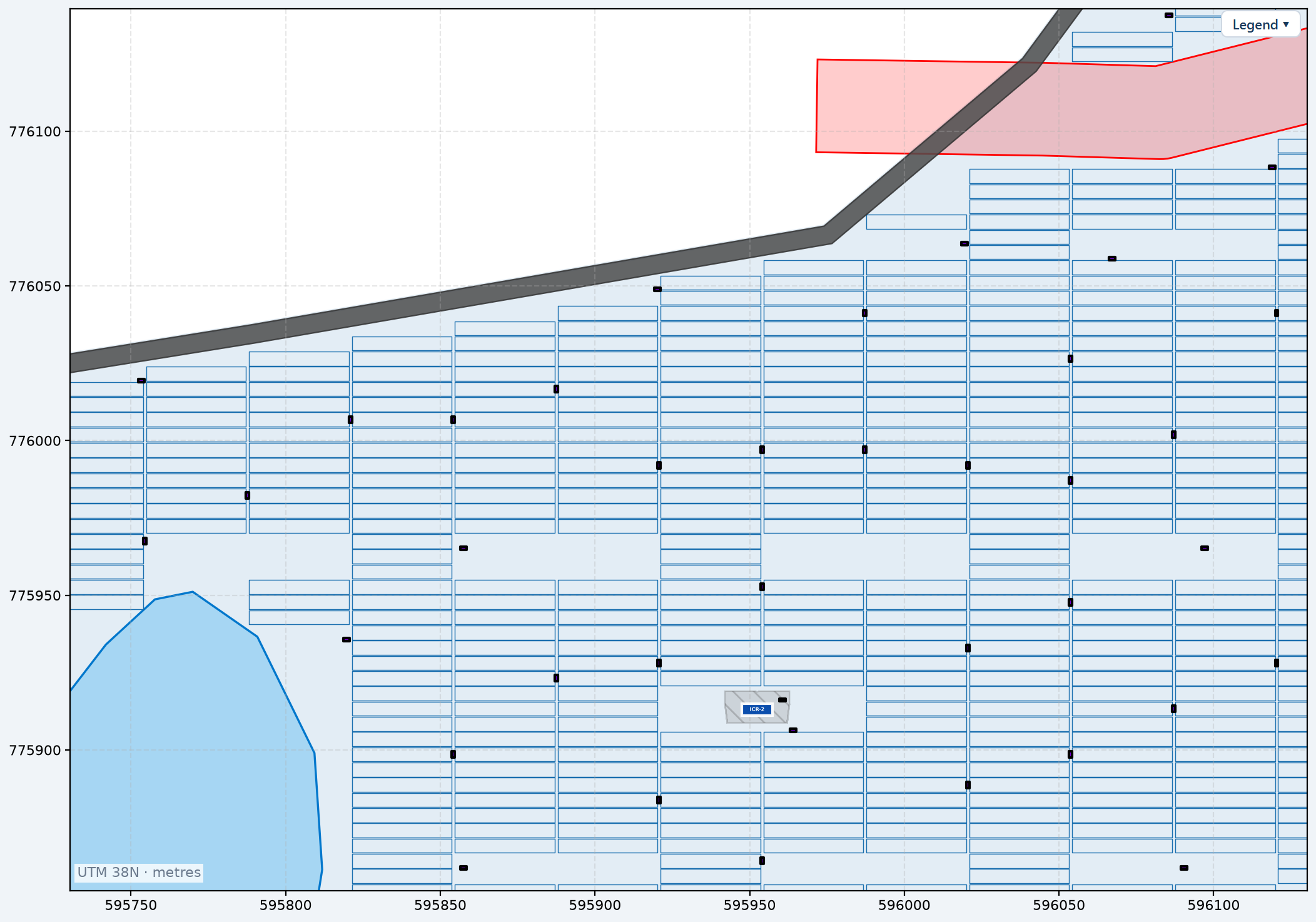
| Wireframe | Off — tables are drawn filled | Draws tables and tracker units as outlines only |
| Piles: OFF | Off, and disabled until a layout exists | Shows the pile overlay; the first use opens the Pile layout window. See Pile layout |
| Layers ▾ | — | Opens the popover of on/off rows, below |
| Sketch | Off | Switches Sketch Mode on. See Sketch Mode |
| Home, Pan, Zoom | — | Fit the whole plant; drag to move the view; drag a box to zoom into it |
| Expand | — | Opens the plot in a window of its own |
Satellite is the fastest check that a layout is standing on the ground you meant. Real tracks, ponds and buildings appear behind the tables, so a missing obstruction in the boundary file is obvious.
Wireframe is the view to use when tables are dense enough to merge into a solid block of colour, and when you want to see cables or piles that filled tables would otherwise hide.
When the window is too narrow for every tool, Satellite, Wireframe and Piles move to the top of the Layers popover as rows of their own and the button reads Layers ▾ +3. Nothing is lost; it has moved.
The Layers popover
Layers ▾ opens a popover of ON/OFF rows, each controlling one layer of the drawing.
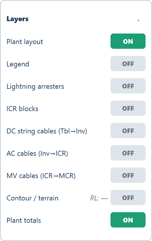
| Row | Default | What it shows |
|---|---|---|
| Plant layout | ON | The tables and equipment. Off leaves only the boundary and obstacles |
| Legend | OFF | The colour key on the plot — the same switch as the Legend ▾ chip in the plot corner |
| Lightning arresters | OFF | The arrester rectangles, their labels and their protection circles |
| ICR blocks | OFF | Each control room's block of tables, filled in its own colour and outlined |
| DC string cables (Tbl→Inv) | OFF | Enabled only when cables were calculated |
| AC cables (Inv→ICR) — DC cables (SMB→CI) in a central-inverter design | OFF | Enabled only when cables were calculated |
| MV cables (ICR→MCR) | OFF | Needs a main control room placed and cables calculated |
| Contour / terrain | OFF | Elevation contours, with a readout of the RL range and the excluded area |
| Plant totals | ON | The row of plant chips under the view; off hides it |
The three cable rows and the arrester row start off because a first run usually has neither cables nor arresters to draw. Switch them on after a run that produced them.
The colour key
The legend is folded by default so it never sits on the drawing. Open it from the Legend ▾ chip in the plot's top-right corner — or from the Legend row of the popover, which is the same switch — and the chip reads Legend ▴ while it is open. The open legend can be dragged out of the way.
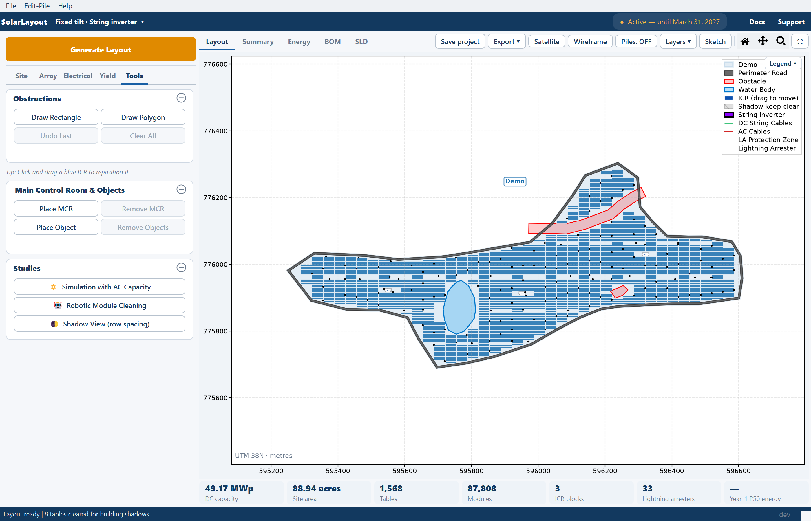
The colours are fixed:
| Drawn in | What it is |
|---|---|
| Blue | Module tables and tracker units |
| Dark blue | Inverter control rooms |
| Violet | The main control room, and the string inverters |
| Green | DC string cables |
| Red | AC cables |
| Dark green | Medium-voltage cables between the control rooms and the main control room |
| Orange-red | Lightning arrester protection circles |
| Red | Obstructions, exclusion zones and transmission line corridors |
| Blue | Water bodies |
| Grey | The perimeter road band |
Contour lines, when the Contour / terrain row is on, run green at the lowest elevation through blue to red at the highest, and the excluded area is reported in acres.
The plot also carries a units note in its bottom-left corner naming the UTM zone and the unit — metres — so a drawing captured from the screen says what its coordinates are.
Moving around the plot
The mouse wheel zooms at the cursor, so pointing at a control room and rolling the wheel takes you straight to it. Pan drags the view and Zoom drags a box to zoom into; Home fits the whole plant again, whatever you have panned or zoomed to — it does not step back through earlier views.
The view you set persists. The plot keeps your zoom and position across redraws — switching a layer on, moving a control room, drawing an obstruction — until you click Home, generate a new layout or load a new boundary file.
For anything you need to look at closely, the expand button at the right of the tools opens SolarLayout — Expanded View: the plot in a large, resizable window with a full toolbar. ⟵ Return to Main Window brings the plot back; until you do, the main window says so in the plot's place.
The plant chips
A row of chips under the view carries the plant totals — DC capacity, site area, tables or trackers, modules, ICR blocks, lightning arresters once some are placed, and year-one P50 energy once it has been calculated. They are the only place the totals appear; the status bar no longer carries them. Clicking a chip opens the Summary view, which replaced the table that used to sit under the plot and holds every per-plant figure. Every row of it is defined in Summary rows.
Where to go next
Views
The five views, their tools and the chip row under them
Maximizing placement and half tables
The two options that trade a regular grid for capacity
Inverter control rooms
How many there are, where they go, and moving one by hand
Site parameters
Perimeter road, capacity block, corridor and arrester radius
String sizing
The String sizing window opened from the Size… button — the three voltage limits that bound the number of modules in series, what you enter, and where the result lands.
Maximizing placement and half tables
Two options that fit more capacity onto an awkward boundary, what each costs in regularity, and when a regular plant is worth more than the extra tables.