How yield is calculated
The energy model — in-plane irradiance, performance ratio, specific yield, degradation, capacity factor — the Yield tab that runs it, and the Energy view that shows the result.
The energy calculation turns one irradiance figure and one performance ratio into an annual generation number, then degrades that number across the plant lifetime and reports it at three exceedance probabilities. Every step is a single explicit relation, and every input to those relations is either a field you can see on the Yield tab or a value fetched and displayed on screen. Nothing in the chain is hidden, which is what makes the output defensible.
This page is the whole chain in order, the controls that run it, and every place the result appears. The sub-pages hold the detail behind each link in the chain.
What the calculation needs before it can run
Two things, and it will not produce a yield without either.
A generated layout. Plant capacity in kWp is the placed module count multiplied by the module wattage, so it does not exist until placement has run. See Your first layout. Everything else in the chain is a per-kWp figure that only becomes energy when it is multiplied by that capacity.
A site position. Latitude and longitude decide the solar geometry, the irradiance the weather source returns, the automatic tilt and the automatic row pitch. A Google Earth boundary file carries the position inside it. A CAD drawing and a raster image do not.
A CAD or image boundary loaded without a site latitude and longitude still produces a layout — the geometry is complete and the summary fills in — but energy calculation is unavailable, and the Energy view says so in place of its Calculate energy button. Enter the coordinates when the application asks for them. See CAD boundary and Image boundary.
The Yield tab
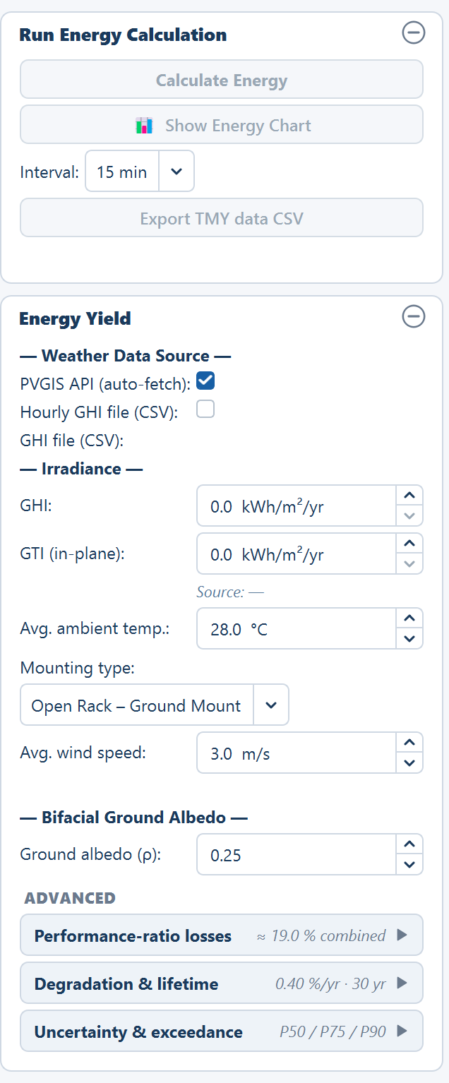
Everything the calculation reads sits on the Yield tab of the inputs, in two cards. The first runs the calculation; the second holds its inputs.
Run Energy Calculation
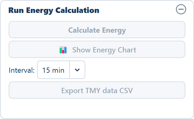
The card is greyed out until a layout exists.
| Control | What it does |
|---|---|
| Calculate Energy | Runs the whole chain below. With the automatic weather source selected, this is also the moment the irradiance is fetched. |
| 📊 Show Energy Chart | Opens the hourly and monthly chart window built from the same series the calculation used. See Charts and time series. |
| Interval: | The time step of the export beside it: 1 min, 10 min, 15 min, 30 min or 1 hour. Ships at 15 min. |
| Export TMY data CSV | Writes a full-year time series of horizontal irradiance, in-plane irradiance and energy at the chosen interval. |
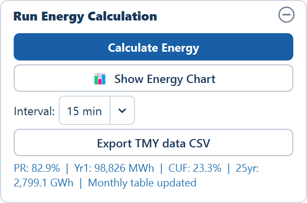
Under the buttons a status line reports what the run is doing and, when it has finished, what it found.
TMY is a typical meteorological year — a single representative year rather than a specific calendar year. The export needs an hourly series to work from, which means either a loaded hourly file or an hourly fetch from the automatic service; an annual total on its own is not enough.
Energy Yield
The second card holds the inputs, top to bottom: the weather source and the irradiance figures, the site conditions the thermal model needs, the ground albedo, and then an ADVANCED block of three expanders. The expanders are collapsed when the tab opens, and each header carries a live one-line summary of what is inside it, so the defaults are visible without opening anything.
| Expander | Header summary on the defaults | Detail |
|---|---|---|
| Performance-ratio losses | ≈ 19.0 % combined | The loss breakdown |
| Degradation & lifetime | 0.40 %/yr · 30 yr | Lifetime, degradation and P-values |
| Uncertainty & exceedance | P50 / P75 / P90 | Lifetime, degradation and P-values |
The weather source and the irradiance fields are on Weather data; the ambient temperature, mounting type and wind speed on Temperature loss; the albedo on Bifacial modules.
Running it
Generate the layout
Capacity comes from the placed modules, so Generate Layout comes first. The computed shading loss is also produced in that pass — see Row-to-row shading.
Click Calculate Energy
On the Yield tab, or on the Energy view, whose gold Calculate energy button is the same action. With the automatic source selected the status line reads "Fetching irradiance from PVGIS…" and then reports what came back, or "PVGIS fetch failed — check your internet connection, or switch to 'Hourly GHI file (CSV)' and load a local file."
Read the status line
When the run finishes the line under the buttons reports the performance ratio, the year-one energy, the capacity factor and the lifetime total, and notes that the monthly table has been updated. The full result is on the Energy view.
The chain, in order
1. In-plane irradiance
The calculation starts from GTI — global tilted irradiance, the annual irradiation arriving on the plane of the modules, in kWh/m²/yr. It is not the same quantity as GHI, global horizontal irradiance, which is what most weather records contain. GTI is the one that drives the yield.
Where GTI comes from depends on your weather source: the automatic service returns it directly for your position, tilt and orientation, and an hourly file either carries it or has it derived from the horizontal figure. See Weather data.
2. Performance ratio
PR, the performance ratio, is the fraction of the energy a plant would produce if every module ran at its nameplate efficiency that it actually delivers to the grid. It is a dimensionless number below 1, and it carries every loss between the light hitting the glass and the energy leaving the plant: inverter conversion, cable resistance, soiling, module temperature, mismatch, shading, availability, transformer and the rest.
You do not enter PR. You enter the components, and PR follows from them — the components are combined multiplicatively, as a product of the factors and of one minus each loss, not as one minus their sum. The full relation, component by component, is on The loss breakdown.
3. Specific yield
Specific yield = GTI (kWh/m²/yr) × PRSpecific yield is annual energy per unit of installed DC capacity, in kWh/kWp. It is the figure to compare two designs on the same site with, because it is independent of how big the plant is.
4. Year-one energy, before first-year degradation
Year 1 energy = capacity_kWp × specific yieldcapacity_kWp is the plant's installed DC capacity — the DC capacity (MWp)
row of the Summary view and the DC capacity chip, in kWp. The product is in
kWh; the application reports MWh.
This figure is the plant before any degradation has been applied. It is not a number you will see reported on its own; it is the base the next two relations work from.
5. First year, after first-year degradation
Year 1 (actual) = Year 1 × (1 − first-year degradation %)1st year degradation ships at 1.0 % and accepts 0–10 %. It stands for the loss a module takes in its first year of exposure that it never recovers — principally LID, light-induced degradation. It is separated from the annual figure because it is a one-off step, not a rate.
Year 1 (actual) is the year-one energy every reported figure is built from:
the three probability rows, the capacity factor, and the lifetime total.
6. Every year after the first
Year n (n ≥ 2) = Year 1 (actual) × (1 − annual degradation %)^(n−1)Annual degradation ships at 0.4 %/yr and accepts 0–5 %/yr. It
compounds: the exponent is n − 1, so year 2 has taken one year of
degradation and the final year of a 30-year plant has taken 29.
Plant lifetime ships at 30 years and accepts 1–50. It sets how far the series runs.
7. Capacity factor
CUF = Year 1 (actual) / (capacity_kWp × 8760) × 100 %CUF, the capacity utilisation factor, is year-one energy expressed as a percentage of what the plant would generate if it ran at full DC nameplate output for every hour of the year. 8760 is the number of hours in a year.
Two things follow from the relation, and both matter when someone challenges the figure. It is computed on year one after degradation, not on the before-degradation figure, and it is computed against DC capacity, not AC. A capacity factor quoted against AC capacity on the same plant is a larger number and is not this number.
Degradation, worked from the shipped defaults
The degradation part of the chain can be worked end to end from defaults alone, so it is worth seeing once. The table below is the output multiplier relative to the before-degradation year-one energy, at 1.0 % first-year degradation and 0.4 %/yr annual degradation.
| Year | Relation | Multiplier |
|---|---|---|
| 1, before degradation | — | 1.000 |
| 1, actual | 1 − 0.010 | 0.990 |
| 2 | 0.990 × 0.996 | 0.986 |
| 10 | 0.990 × 0.996⁹ | 0.955 |
| 30 | 0.990 × 0.996²⁹ | 0.881 |
The last row is the one a lender's model usually wants: on the shipped defaults, the final year of a 30-year plant generates about 88.1 % of what year one would have generated before any degradation at all.
The first three steps of the chain cannot be worked the same way, and it is worth being clear about why rather than picking plausible numbers. GTI (in-plane) ships at 0.0 until a weather source fills it, and capacity comes from your own placed layout — so any absolute MWh example would be an invented site, not a default. Run the chain on your own site instead.
See Lifetime, degradation and P-values for how the same series is turned into the exceedance probabilities.
Monthly figures
Alongside the annual numbers the application produces a month-by-month table following IEC 61724-1, the standard for PV system performance monitoring. Three quantities per month:
Y_r  = H_i / G_STC          reference yield, in hours
Y_f  = E_AC / P_0           final yield, in kWh/kWp
PR_m = Y_f / Y_r monthly performance ratioH_iis the month's in-plane irradiation andG_STCthe standard test condition irradiance, soY_ris the number of equivalent full-sun hours in the month.E_ACis the month's AC energy andP_0the installed DC capacity, soY_fis the month's specific yield.PR_mis their ratio — the same definition as the annual PR, evaluated on one month.
Monthly PR is not the annual PR repeated twelve times. It moves with module temperature, and module temperature moves with the month's ambient temperature and its own operating irradiance:
G_m = monthly GTI × 1000 / (days × 8 h/day) W/m²Monthly ambient temperature comes from a sinusoidal seasonal model whose amplitude scales with the absolute latitude of the site — or, when your weather file carries a temperature column, from the file itself. The module temperature for the month then follows the Sandia relation on Temperature loss. A hot low-latitude site therefore shows its lowest monthly PR in the hottest months, which is the behaviour a reviewer expects to see.
The Energy view
The result lives on the Energy view, one of the five view tabs on the right of the window — see Views for the tabs and the tools beside them. If the result lands while another view is showing, the tab reads Energy • until you open it.
Before a run
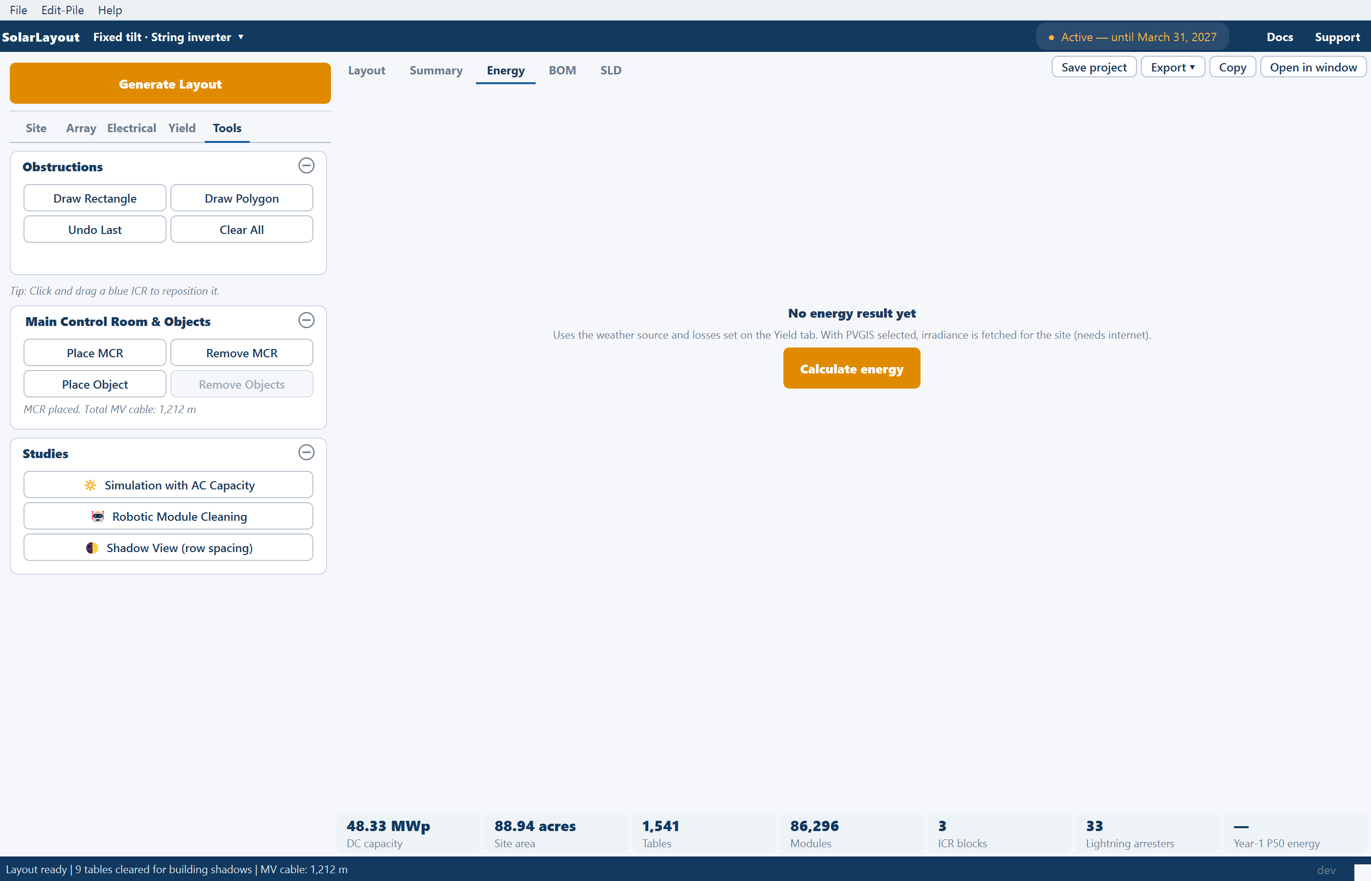
The view opens with the title No energy result yet and a note that says what is missing. Before a layout it reads "Generate a layout first. Energy is calculated for the generated layout."; once a layout exists it reads "Uses the weather source and losses set on the Yield tab. With PVGIS selected, irradiance is fetched for the site (needs internet).", over a gold Calculate energy button that does what the Yield tab's button does.
After a run
Four tiles across the top carry the annual answer:
| Tile | Unit | What it is |
|---|---|---|
| Year-1 energy | MWh | Year 1 (actual) from step 5 |
| Specific yield | kWh/kWp | Step 3 |
| Performance ratio | % | Step 2 |
| CUF | % | Step 7 |
Under them is the monthly table, titled "Monthly Energy Breakdown — IEC 61724-1 — Year 1 (all plants combined)": twelve rows and a TOTAL / Annual row, in these columns:
| Column | What it holds |
|---|---|
| Month | January to December |
| GHI (kWh/m²) | Horizontal irradiation for the month |
| H_i (kWh/m²) | In-plane irradiation for the month |
| T_amb (°C) | The month's ambient temperature, from the seasonal model or your file |
| T_cell (°C) | The month's module temperature from the Sandia relation |
| Y_r (h) | Reference yield — equivalent full-sun hours |
| Y_f (kWh/kWp) | Final yield — the month's specific yield |
| PR (%) | The monthly performance ratio |
| Energy (MWh) | The month's generation |
| CUF (%) | The month's capacity factor |
Two charts complete the view: In-plane irradiation (kWh/m², bars) and performance ratio (%, line) under the table, and Monthly energy, Year 1 (MWh) on the right. On a short window the irradiation chart steps aside to keep the table readable.
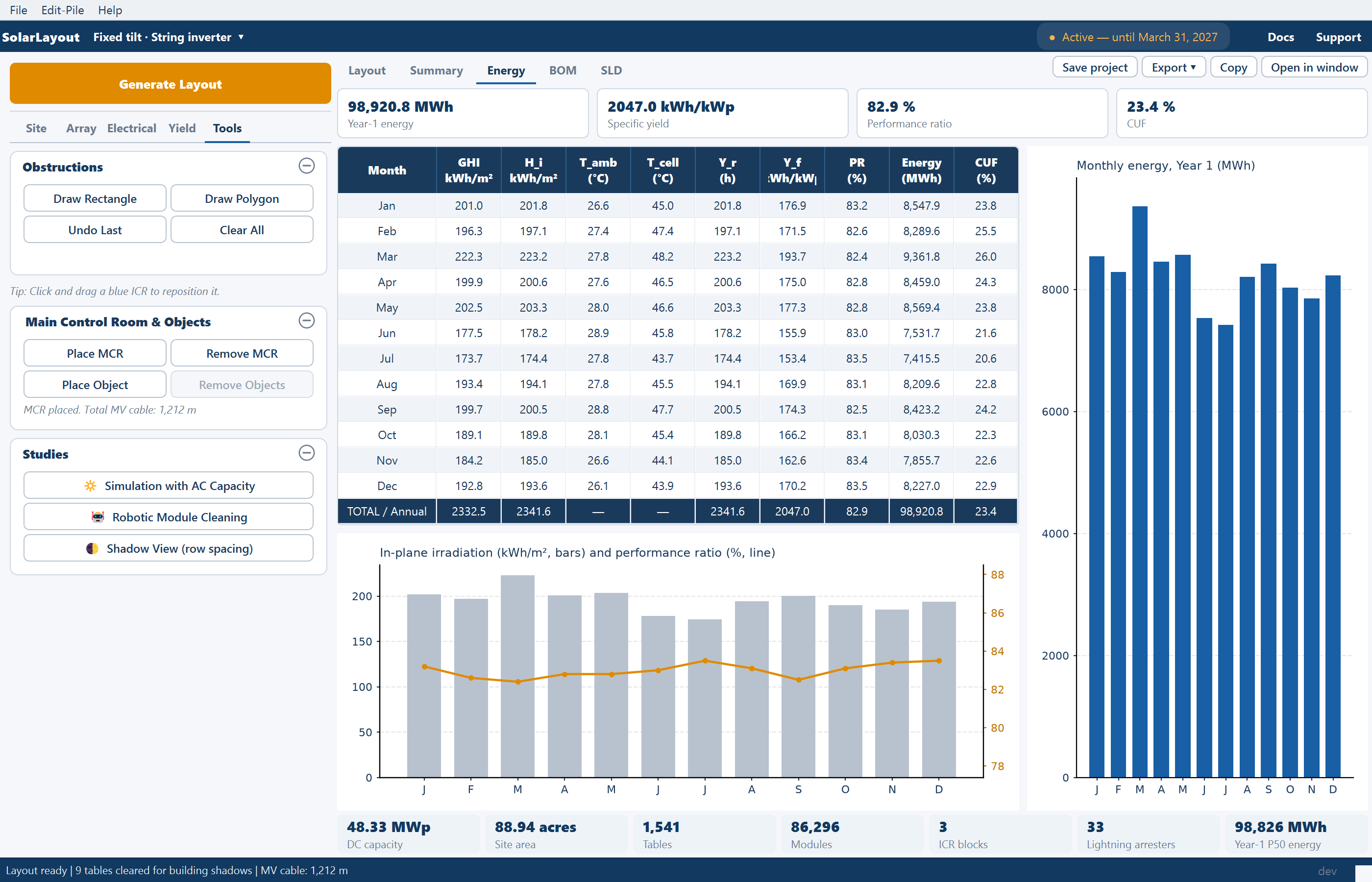
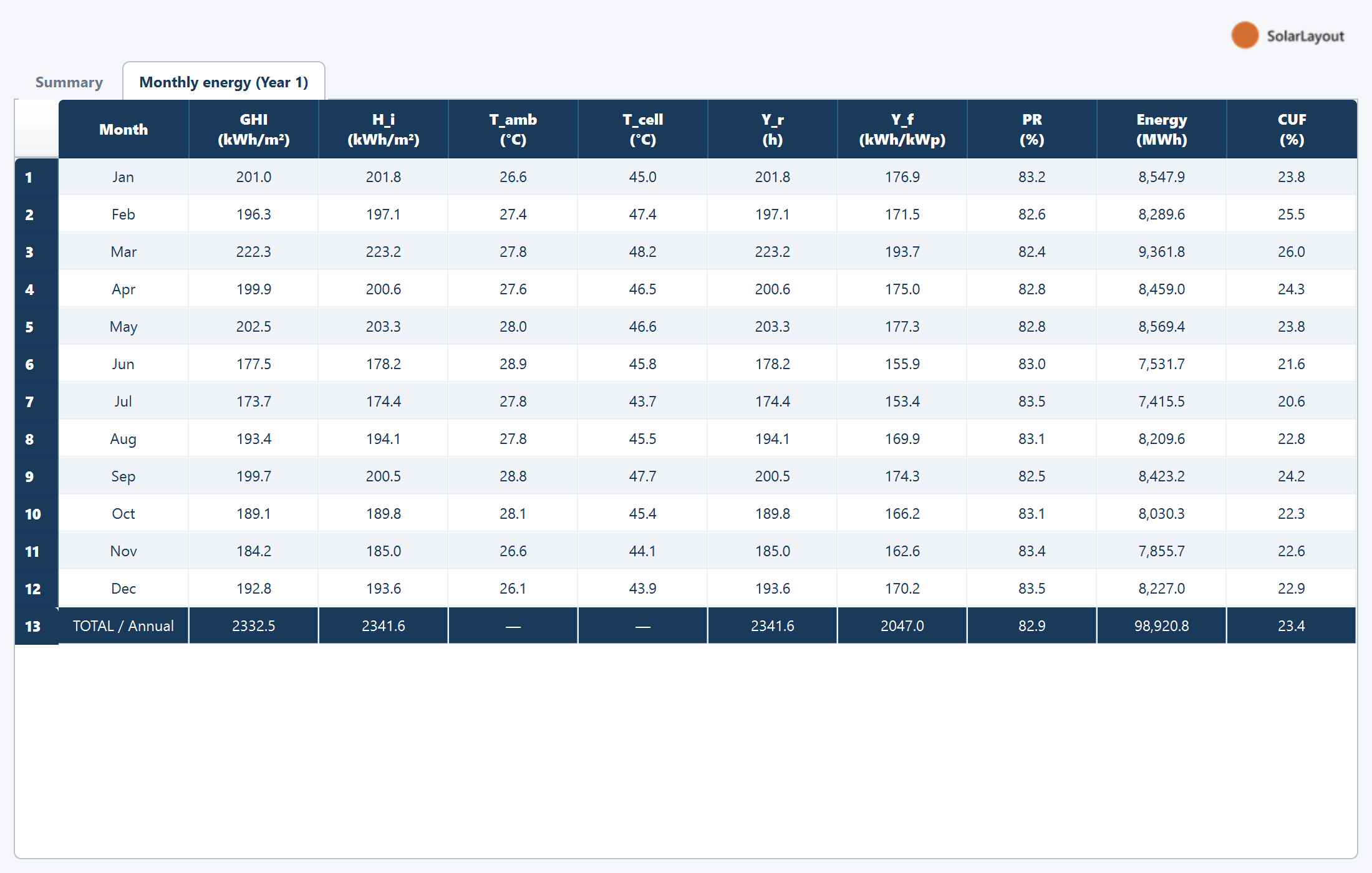
The view's tools, right of the view tabs, are Copy and Open in window. The second opens SolarLayout — Summary, a separate window whose Monthly energy (Year 1) tab holds the same table and follows the layout as it changes, so it can sit beside the plot on a second screen.
Where else the result appears
The Summary view. Its ENERGY group carries five rows, one column per
plant. Before a run they read —.
| Row | What it holds |
|---|---|
| P50 energy, year 1 (MWh) | Year-one energy at the first exceedance probability |
| P75 energy, year 1 (MWh) | Year-one energy at the second |
| P90 energy, year 1 (MWh) | Year-one energy at the third |
| CUF (%) | The capacity factor from the relation above |
| P50 energy, 25 years (MWh) | The lifetime total — every year from 1 to Plant lifetime, summed, at the first probability. The "25 years" in the name is fixed text and does not follow the setting. |
The three probability rows are named from your own settings. They read P50 / P75 / P90 because Exceedance prob. 1, 2 and 3 ship at 50.0, 75.0 and 90.0 %. Change any of them and the row name changes with it. Two results are therefore only comparable row for row if both were run with the same three probabilities — check the names, not the position.
The two lower probabilities are derived from the first through the combined uncertainty:
P75 = P50 × (1 − 0.674 × σ)
P90 = P50 × (1 − 1.282 × σ)
σ is Combined uncertainty (1σ), which ships at 5.0 % and accepts
0.1–30.0 %. The multipliers are the standard normal deviates at those
exceedance levels.
The last row is mislabelled — the figure is not a 25-year one. The row reads P50 energy, 25 years (MWh) whatever the lifetime is set to, while the value beside it is the sum of every year from 1 to Plant lifetime, scaled to the first exceedance probability. On the shipped default lifetime of 30 years, the row named "25 years" therefore reports a 30-year total. Unlike the three probability rows, this one does not follow its own setting. Quote the figure as the lifetime total and state the lifetime you used alongside it.
The plant chips. The row under every view carries a Year-1 P50 energy
chip — — before a run — which opens the Energy view when clicked. It is the
only place the total is shown outside the views; the status bar never carries
it.
The Yield tab's status line. After a run it reports the performance ratio, the year-one energy, the capacity factor and the lifetime total in one line — the same lifetime figure as the Summary row, labelled with the same fixed "25yr".
The Word report. Export ▾ Export Detailed Project Report writes an Energy Yield & Loss Analysis section and an Energy Yield — Drawings annex, present only when energy has been calculated. See Project report. The full Summary row set is on Summary columns.
What this model is and is not
State these plainly to anyone reviewing the output, because they are the questions a careful reviewer asks.
It is a yield estimate from a loss model, not an hourly plant simulation. The annual result is an annual irradiation total multiplied by a single performance ratio and a capacity. Hourly data is used — for the transposition from horizontal to in-plane irradiance, for the shading loss, and for the charts and the export — but the energy figure is not an hour-by-hour simulation of module, inverter and transformer behaviour, and it does not replace one.
Row-to-row shading is modelled; terrain and horizon shading are not. The near-shading loss is computed from your own row geometry, and tables falling inside the year-round shadow of a structure you place are cleared from the layout. Distant horizon profiles and shading from the site's own relief are not part of the model. See Row-to-row shading.
The result is only as good as the weather data behind it. Every number on this page is downstream of one irradiance figure. A monthly climatology average and a purchased site-specific typical meteorological year will not give the same answer, and the difference between them is larger than most of the loss components you might argue about. Check which source produced your irradiance before quoting the yield — the source line on the Yield tab names it.
The energy pages
Weather data
The automatic service, your own hourly file, and how horizontal irradiance becomes in-plane
The loss breakdown
Every component of the performance ratio, with defaults and ranges
Temperature loss
The thermal model, the four mounting types, and why this loss is computed rather than assumed
Row-to-row shading
Near-shading from your own geometry, and the Shadow View
Bifacial modules
Ground albedo and how rear-side irradiance is estimated
Lifetime, degradation and P-values
Degradation, plant lifetime, uncertainty and the exceedance probabilities
Charts and time series
The chart window, and the time-series export
Where to go next
Pile layout
Define a pile pattern on one reference table in the Pile layout window, stamp it onto every table in the plant, and export the coordinates a setting-out team works from.
Weather data
The automatic irradiance service and its fallback, your own hourly file and what it must contain, and how horizontal irradiance becomes in-plane.